

Two routes to work both take about 28 minutes on a normal day. One of them makes you late twice every two weeks. The other never does. An average can’t tell them apart. The interquartile range can.
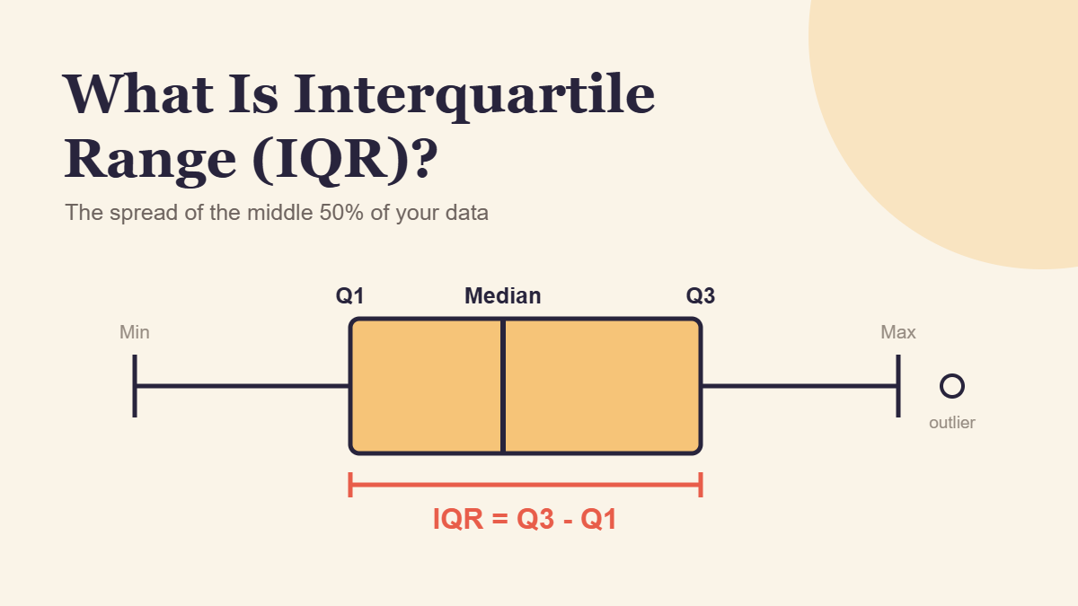
The interquartile range (IQR) is the spread of the middle 50% of a data set. You get it by subtracting the first quartile (Q1) from the third quartile (Q3). A small IQR means the typical values sit close together. A large one means even “normal” results vary a lot.
This guide shows you how to calculate the IQR, how to read whether it’s big or small, why a typo can wreck a standard deviation but barely touch the IQR, and what the IQR reveals about real US paychecks in 2026.
Quick Info
| Topic | Detail |
|---|---|
| Short definition | The distance between Q1 and Q3, covering the middle 50% of sorted data |
| Formula | IQR = Q3 minus Q1 |
| Units | Same units as the data (minutes, dollars, points) |
| Best for | Skewed data, data with outliers, comparing the consistency of two groups |
| Main limitation | Ignores the lowest and highest 25%, so it says nothing about the extremes |
| Built from it | Outlier fences (Q1 minus 1.5 x IQR, Q3 plus 1.5 x IQR) and box plots |
| Reading time | About 10 minutes |
What Is the Interquartile Range?
The interquartile range is the difference between the third quartile and the first quartile, and it measures how spread out the middle half of your data is.
Picture a group photo where everyone lines up from shortest to tallest. Crop off the shortest quarter and the tallest quarter. The height difference between the shortest and tallest person still in the picture is, roughly, the IQR.
If you need a refresher on Q1 and Q3 themselves, our guide to quartiles in statistics walks through finding them by hand and explains why Excel sometimes disagrees with your calculator. This article picks up from there and focuses on what the IQR does once you have it.
IQR vs Range at a Glance
The range and the IQR both measure spread, but they look at very different parts of the data.
| Range | Interquartile range | |
|---|---|---|
| Formula | Maximum minus minimum | Q3 minus Q1 |
| Values it depends on | The two most extreme values | The two values at the 25% and 75% marks |
| What it describes | Full spread, best to worst | Spread of the typical middle half |
| Effect of one wild value | Can change it enormously | Usually little or no change |
| Good question it answers | “What’s the widest gap we’ve seen?” | “How consistent is a normal result?” |
The Interquartile Range Formula
IQR = Q3 - Q1- Q3 is the upper quartile, the value that about 75% of the data falls at or below.
- Q1 is the lower quartile, the value that about 25% of the data falls at or below.
Because it’s a subtraction of two data values, the IQR always comes out in the same units as your data. An IQR of 6 in a list of commute times means 6 minutes, not 6%.
You’ll also see the semi-interquartile range (or quartile deviation), which is simply half the IQR: (Q3 minus Q1) / 2. It’s the typical distance from the median to either quartile.
How to Find the IQR in 4 Steps
- Sort the values from smallest to largest.
- Find the median and split the list into a lower half and an upper half. With an odd count, leave the median out of both halves.
- Find Q1 and Q3, the medians of the lower and upper halves.
- Subtract: IQR = Q3 minus Q1.
In a spreadsheet, =QUARTILE.INC(A2:A11,3)-QUARTILE.INC(A2:A11,1) does it in one line. On small data sets the answer can differ slightly from a hand calculation, so match whatever method your class or report uses.
Worked Example: Which Commute Route Is More Reliable?
Maya can drive to work on the highway (Route A) or on back roads (Route B). She timed each route on 10 workdays, in minutes. (The figures are illustrative.)
Route A: 24, 26, 22, 31, 25, 55, 27, 29, 28, 48
Route B: 28, 27, 30, 28, 29, 31, 27, 29, 30, 28
Step 1: Sort Each List
Route A: 22, 24, 25, 26, 27, 28, 29, 31, 48, 55
Route B: 27, 27, 28, 28, 28, 29, 29, 30, 30, 31
Step 2: Split Into Halves
Each route has 10 times, so each list splits into two groups of five.
| Route | Lower half | Upper half |
|---|---|---|
| A | 22, 24, 25, 26, 27 | 28, 29, 31, 48, 55 |
| B | 27, 27, 28, 28, 28 | 29, 29, 30, 30, 31 |
Step 3: Find Q1 and Q3
The middle (3rd) value of each half is its quartile.
Route A: Q1 = 25, Q3 = 31
Route B: Q1 = 28, Q3 = 30
Step 4: Subtract
Route A: IQR = 31 - 25 = 6 minutes
Route B: IQR = 30 - 28 = 2 minutes
Step 5: Make the Call
The medians are almost identical: 27.5 minutes for Route A and 28.5 for Route B. If Maya only looked at the typical time, she’d call it a tie.
The IQR breaks the tie. On a normal day, Route B lands inside a 2-minute window. Route A wanders across 6 minutes, and that’s before counting the two traffic-jam days (48 and 55 minutes) that the IQR deliberately sets aside.
If Maya has a 9:00 meeting she can’t miss, Route B is the smarter pick, even though it’s a minute slower on a typical day. That’s the IQR’s real job: telling you how much you can count on the typical result.
Real Example: The IQR of US Weekly Paychecks
The IQR isn’t just a classroom number. Every quarter, the Bureau of Labor Statistics publishes the first quartile, median and third quartile of weekly pay for full-time workers. In its third-quarter 2026 earnings table, the middle half of all full-time wage and salary workers earned between $849 and $1,908 a week. That’s an IQR of $1,059.
Subtract Q1 from Q3 for each group in the same table and the spread tells its own story.
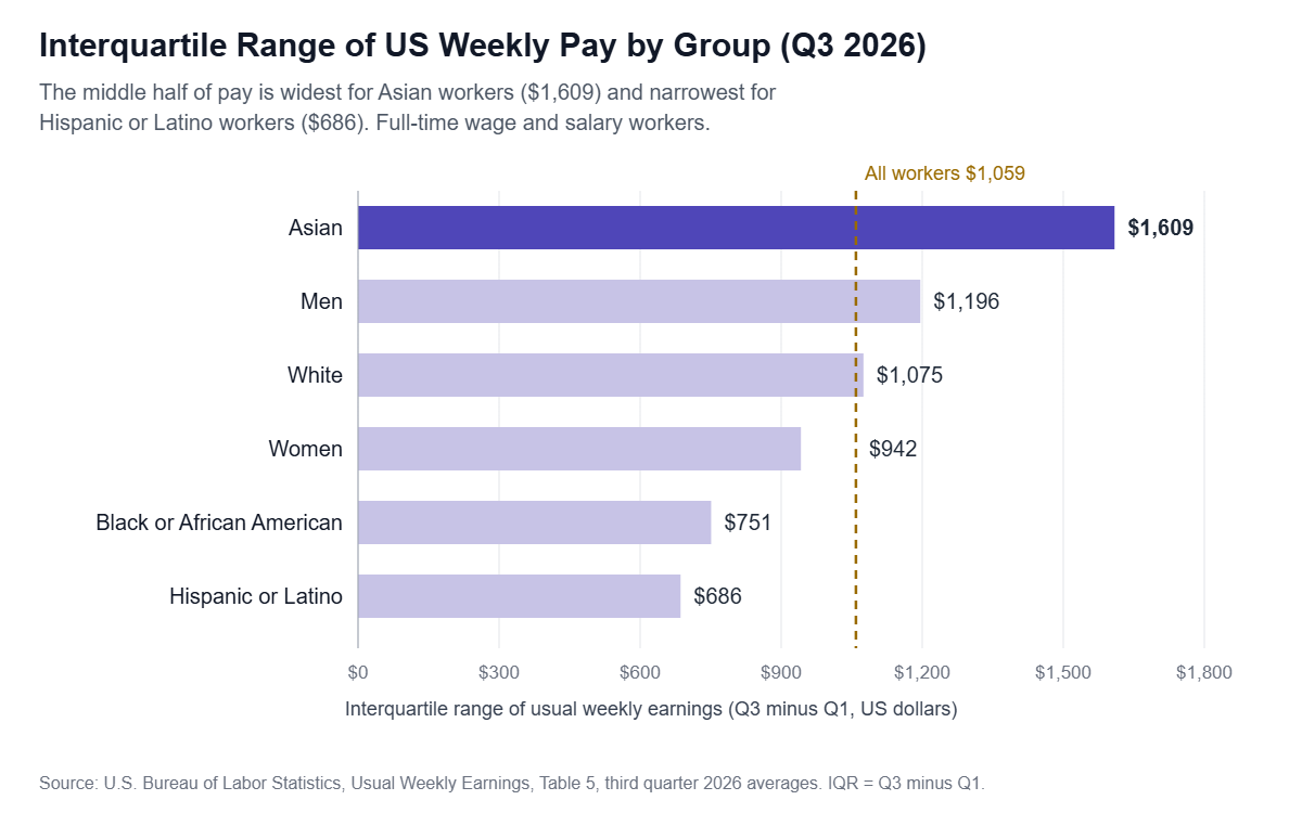
The middle half of Asian workers spans $1,609 a week, more than double the $686 spread for Hispanic or Latino workers. A wide IQR here means a typical worker in that group could be earning very different amounts, while a narrow IQR means typical pay is bunched together.
Is an IQR of $1,059 Big or Small?
On its own, a raw IQR is hard to judge. A $1,000 spread is huge for a group earning $500 a week and modest for one earning $5,000. A quick fix is to compare the IQR to the median:
Relative spread = IQR / medianFor all workers, $1,059 divided by $1,232 is about 0.86. For Hispanic or Latino workers it’s about 0.70, and for Asian workers it’s about 0.99. Even after adjusting for the size of typical pay, Asian workers’ earnings are the most spread out of these groups.
One caution: these figures describe how pay is spread within each group. On their own, they don’t explain why, since occupation, age, education and location all differ between groups.
Why the IQR Shrugs Off Outliers (and Standard Deviation Doesn’t)
Penn State’s introductory statistics course calls the IQR a resistant measure: only a few values decide it, and none of them are the extreme ones. Standard deviation is the opposite, a sensitive measure, because every value feeds into it.
You can watch this happen with one typo. Say Maya logs Route B’s 31-minute day as 310 by accident.
| Measure for Route B | Correct data | With the 310 typo | Change |
|---|---|---|---|
| Median | 28.5 min | 28.5 min | None |
| IQR | 2 min | 2 min | None |
| Mean | 28.7 min | 56.6 min | Nearly doubles |
| Standard deviation | 1.34 min | 89.04 min | About 66 times larger |
| Range | 4 min | 283 min | About 70 times larger |
One bad keystroke turned a 2-minute-wide route into a “wildly unpredictable” one, according to the standard deviation and range. The IQR didn’t move at all, because the typo landed in the top quarter, which the IQR ignores.
When to Use the IQR vs Standard Deviation
The same Penn State lesson gives a simple rule: use resistant measures like the IQR when a sample has outliers or skewness, and sensitive measures like standard deviation when it’s reasonably symmetric.
| Your data looks like… | Use | Report it with |
|---|---|---|
| Roughly symmetric, no extreme values (heights, many test scores) | Standard deviation | The mean |
| Skewed to one side (incomes, home prices, wait times) | IQR | The median |
| Has a few extreme values you can’t remove | IQR | The median |
| You need it for further formulas (confidence intervals, z-scores) | Standard deviation | The mean |
A handy cross-check: for data that’s close to bell-shaped, the IQR comes out at about 1.35 times the standard deviation. If your IQR is far smaller or larger than that, your data probably isn’t bell-shaped, and the IQR is likely the safer summary.
Using the IQR to Flag Outliers
The IQR also sets the boundaries for what counts as “unusual.” Multiply it by 1.5 and stretch that distance past each quartile:
Lower fence = Q1 - 1.5 x IQR
Upper fence = Q3 + 1.5 x IQR
For Route A, the IQR is 6, so 1.5 x 6 = 9:
- Lower fence: 25 minus 9 = 16 minutes
- Upper fence: 31 plus 9 = 40 minutes
The 48- and 55-minute days both sit above 40, so they’re flagged as outliers. For Route B, the fences are 25 and 33 minutes, and every one of its 10 days fits inside. That confirms what the IQR already hinted at: Route A has a traffic-jam problem, Route B doesn’t.
On a box plot, the IQR is literally the length of the box, and these fences decide where the whiskers stop.
Common IQR Mistakes
| Mistake | Why it’s wrong | What to do instead |
|---|---|---|
| Calling the IQR “the middle 50% of values” | The IQR is one number, a distance, not a group of values | Say “the spread of the middle 50%” |
| Subtracting the median somewhere | The median isn’t part of the formula | IQR = Q3 minus Q1, nothing else |
| Forgetting to sort | Quartiles from an unsorted list are meaningless | Always sort first |
| Comparing raw IQRs across very different scales | A $1,000 IQR means different things at $500 vs $5,000 | Divide by the median for a relative spread |
| Deleting every value outside the fences | Flags aren’t errors; some are the most important data | Check each flagged value before removing it |
| Assuming a small IQR means no extremes | The IQR ignores the top and bottom 25% entirely | Look at the range or a box plot too |
Frequently Asked Questions
What does the interquartile range tell you?
It tells you how tightly the typical values are packed. A small IQR means the middle half of the data sits close together, so results are consistent. A large IQR means even ordinary results vary a lot. Because it skips the top and bottom quarters, it describes the usual case rather than the extremes.
Can the interquartile range be negative?
No. Q3 is always greater than or equal to Q1, so Q3 minus Q1 is zero or positive. If you get a negative number, you’ve probably subtracted in the wrong order or forgot to sort the data before finding the quartiles.
What does an IQR of zero mean?
It means Q1 and Q3 are the same value, so at least the middle half of your data is identical. That happens with heavily repeated values, like a survey where most people pick the same rating. The data can still have very different values in the top and bottom quarters.
Is the IQR the same as the semi-interquartile range?
No. The semi-interquartile range, also called the quartile deviation, is half the IQR: (Q3 minus Q1) / 2. For Route B in the example above, the IQR is 2 minutes and the semi-interquartile range is 1 minute.
Is a higher or lower IQR better?
Neither is good or bad by itself. A low IQR is great when you want consistency, like delivery times or medication doses. A high IQR may be expected, like incomes across a whole country. Judge it against your goal and against the median, not in isolation.
How is the IQR shown on a box plot?
The IQR is the length of the box. The left (or bottom) edge sits at Q1, the right (or top) edge sits at Q3, and the line inside marks the median. A long box means a wide IQR. Values beyond the 1.5 x IQR fences appear as separate dots.
Conclusion
The interquartile range is Q3 minus Q1, the spread of the middle half of your data. It ignores extreme values on purpose, which makes it the right spread measure for skewed data, data with outliers, and any time you care more about the typical result than the rare one. Pair it with the median, compare it to the median when scales differ, and use 1.5 x IQR to flag values worth a second look.
Next time two options share the same average, don’t stop there. Ask which one has the smaller IQR.
References
- U.S. Bureau of Labor Statistics, “Table 5. Quartiles and selected deciles of usual weekly earnings of full-time wage and salary workers by selected characteristics, third quarter 2026 averages,” released October 21, 2026.
- Penn State Eberly College of Science, STAT 100, “3.5 – Measures of Spread or Variation.”
Disclaimer
This article is for general educational purposes only. The commute times in the worked example are illustrative, and the earnings figures are BLS averages for the third quarter of 2026 that may be revised. For research, grading or business decisions, confirm the quartile method your textbook, instructor or software uses.