

Half of America’s full-time workers earn less than $1,232 a week. That single number is useful, but it hides a lot. Is most of the country bunched close to $1,232, or spread from a few hundred dollars to several thousand?
The Bureau of Labor Statistics answers that with three numbers instead of one. In its third-quarter 2026 earnings table, the middle half of full-time wage and salary workers earned between $849 and $1,908 a week. Those two cutoffs, plus the median, are quartiles.
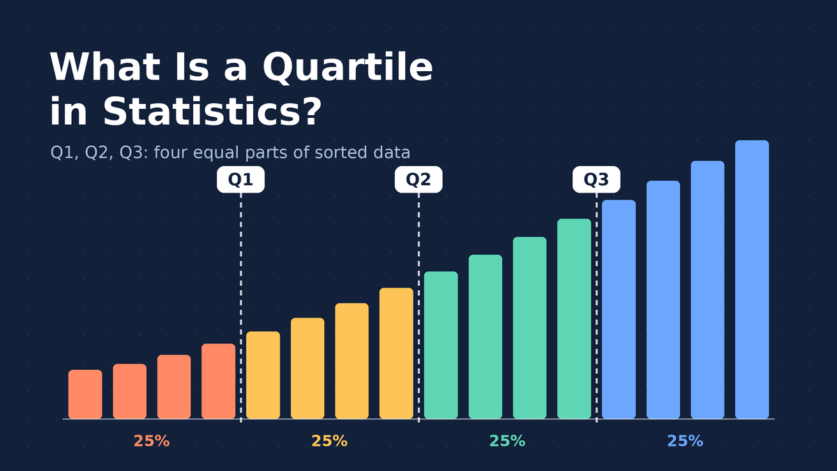
A quartile in statistics is one of three values that split an ordered data set into four equal parts. Once you can find them, you can describe where most of your data sits, how spread out it is, and which values look suspicious.
This guide covers what Q1, Q2 and Q3 mean, how to find them by hand for odd and even data sets, why Excel and your calculator sometimes disagree, and how to use quartiles to spot outliers.
Quick Info
| Topic | Detail |
|---|---|
| Short definition | Three cut points (Q1, Q2, Q3) that split ordered data into four groups of roughly equal size |
| Q1 (lower quartile) | About 25% of values fall at or below it |
| Q2 (median) | The middle value; 50% fall at or below it |
| Q3 (upper quartile) | About 75% of values fall at or below it |
| Key measure built from them | Interquartile range: IQR = Q3 minus Q1 |
| Common surprise | Excel, calculators and textbooks can give slightly different Q1 and Q3 for the same data |
| Reading time | About 10 minutes |
What Is a Quartile?
A quartile is a value that marks one of the three boundaries dividing sorted data into four equal-sized groups.
Think of a line of 100 people sorted by height. Walk 25 people in and stop: that person’s height is roughly Q1. Stop at person 50 and you’re at Q2, the median. Stop at person 75 and you’ve reached Q3.
Here’s the part that trips people up. A quartile is a value, not a group. “Q1” is the single number at the 25% mark. The 25% of people shorter than that number are often called the “first quarter” or “bottom quarter” of the data.
| Name | Also called | Share of data at or below it | What it tells you |
|---|---|---|---|
| Q1 | Lower quartile, 25th percentile | About 25% | Where the low end of “typical” begins |
| Q2 | Median, 50th percentile | About 50% | The middle of the data |
| Q3 | Upper quartile, 75th percentile | About 75% | Where the high end of “typical” ends |
The Five-Number Summary
Add the smallest and largest values to the three quartiles and you get the five-number summary: minimum, Q1, median, Q3, maximum.
Those five numbers say a surprising amount. The distance from minimum to maximum is the range. The distance from Q1 to Q3 shows how wide the middle half is. If the gap between Q2 and Q3 is much bigger than the gap between Q1 and Q2, the data stretches out on the high side, which is called right skew.
Why Not Just Use the Mean?
The mean reacts to every value, including extreme ones. One billionaire moving into a small town raises the average income for everyone on paper. Q1, the median and Q3 barely move, because they depend on position in the sorted list, not on how big the extreme value is.
That’s why salaries, home prices, wait times and test scores are so often reported with quartiles. Those data sets tend to have a long tail on one side.
How to Find Quartiles by Hand
The most common classroom approach is the median-of-halves method. It works in four moves.
- Sort the data from smallest to largest.
- Find the median. That’s Q2.
- Split the data into a lower half and an upper half. If the count is odd, leave the median out of both halves.
- Q1 is the median of the lower half. Q3 is the median of the upper half.
Odd Number of Values
Say you tracked your daily steps (in thousands) for nine days:
4, 6, 7, 8, 9, 10, 11, 13, 15The median is the 5th value, 9, so Q2 = 9. Leave the 9 out. The lower half is 4, 6, 7, 8, and its median is (6 + 7) / 2 = 6.5. The upper half is 10, 11, 13, 15, and its median is (11 + 13) / 2 = 12.
So Q1 = 6.5, Q2 = 9 and Q3 = 12. On a typical day in the middle half, you walked between 6,500 and 12,000 steps.
Even Number of Values
With an even count, the median falls between two values, and the data splits cleanly into two equal halves. Nothing gets left out. The worked example below shows this case from start to finish.
The Position Formula
Some textbooks skip the halves and use positions instead:
Q1 position = (n + 1) / 4
Q2 position = (n + 1) / 2
Q3 position = 3(n + 1) / 4
Here, n is the number of values. The result tells you which place in the sorted list to look at, not the quartile itself. If you get 3.25, the quartile sits one quarter of the way from the 3rd value to the 4th. This method can give slightly different answers from the median-of-halves method, which is exactly why the next section matters.
Worked Example: Pizza Delivery Times
A small pizza shop logs how long its last 12 deliveries took, in minutes. The owner wants to know what a “normal” delivery looks like before promising customers a time. (The figures are illustrative.)
Step 1: Sort the Data
18, 21, 22, 24, 25, 27, 29, 30, 32, 35, 38, 61There are 12 values, so n = 12. Sorting matters more than people think. Run the steps on an unsorted list and every quartile comes out wrong.
Step 2: Find the Median (Q2)
With 12 values, the middle falls between the 6th and 7th values, 27 and 29.
Q2 = (27 + 29) / 2 = 28Half the deliveries took 28 minutes or less.
Step 3: Split Into Halves
Because 12 is even, the list splits cleanly into two groups of six.
| Lower half | Upper half |
|---|---|
| 18, 21, 22, 24, 25, 27 | 29, 30, 32, 35, 38, 61 |
Step 4: Find Q1 and Q3
Each half has six values, so each median is the average of its 3rd and 4th values.
Q1 = (22 + 24) / 2 = 23
Q3 = (32 + 35) / 2 = 33.5
Step 5: Read the Result
The middle half of deliveries took between 23 and 33.5 minutes. That’s a far better promise than “about 30 minutes,” which is roughly the mean (362 / 12 = 30.2). The mean got dragged up by one slow 61-minute order, while Q1, the median and Q3 stayed put.
If the owner promises “under 35 minutes,” Q3 already tells them at least three out of four orders will make it (in this log, 10 of 12 did). That’s the practical power of Q3.
Why Excel and Your Calculator Give Different Quartiles
Run those same 12 delivery times through different tools and you may not get 23 and 33.5. Statisticians never agreed on a single rule for small data sets, so software picks one of several methods.
| Method | Q1 | Q2 | Q3 |
|---|---|---|---|
| Median of halves (by hand, TI-84 style) | 23 | 28 | 33.5 |
| Excel QUARTILE.INC (and the older QUARTILE function) | 23.5 | 28 | 32.75 |
| Excel QUARTILE.EXC, same as the (n + 1)/4 position formula | 22.5 | 28 | 34.25 |
Notice the median never changes. Only Q1 and Q3 drift, and only by a minute or so here.
Fort Hays State University’s open textbook on box plots, quartiles and percentiles points out the same thing: Excel’s inclusive and exclusive functions can return different values from a hand calculation, and the gap is biggest with small data sets.
So which one is right? All of them. If you’re doing homework, use the method your teacher or textbook uses. At work, name the method or the function in your report so anyone can reproduce your numbers. With hundreds or thousands of values, the methods land so close together that it rarely matters.
Real Example: Quartiles of US Weekly Earnings
The BLS reports quartiles every quarter because a single average would badly misdescribe pay. Here’s how the three quartiles compare across education levels for full-time workers age 25 and older.
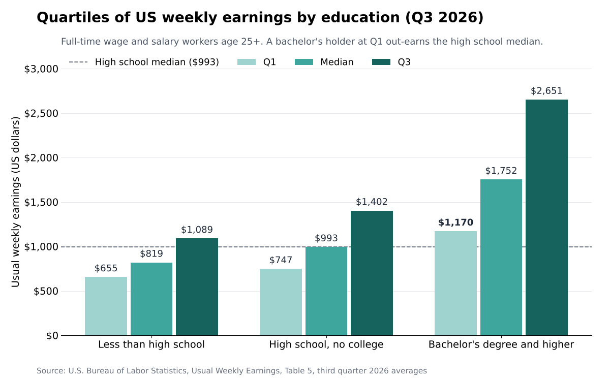
Notice the bachelor’s Q1 bar. A worker at the bottom quarter of that group still earns more each week than the typical high school graduate at the median.
The width of each group’s middle half tells a second story. Subtract Q1 from Q3 and you get the spread of typical pay:
- Less than a high school diploma: $1,089 minus $655 = $434
- High school graduates, no college: $1,402 minus $747 = $655
- Bachelor’s degree and higher: $2,651 minus $1,170 = $1,481
Pay for degree holders isn’t just higher. It’s far more spread out, which makes sense when one group includes both new teachers and surgeons.
One caution: these quartiles describe who earns what. They don’t prove a degree causes the gap on its own, because age, field and location all differ between the groups.
Using Quartiles to Measure Spread: The Interquartile Range
The interquartile range, or IQR, is the distance between Q1 and Q3:
IQR = Q3 - Q1It measures how spread out the middle 50% of the data is. Unlike the range, which uses only the two most extreme values, the IQR ignores the top and bottom quarters entirely. One wild value can’t stretch it.
For the pizza shop, IQR = 33.5 minus 23 = 10.5 minutes. The full range is 61 minus 18 = 43 minutes. Same data, very different picture, because that single 61-minute order inflates the range but leaves the IQR alone.
When your data is roughly bell-shaped, standard deviation is the usual spread measure. When it’s lopsided or has a few extreme values, the IQR usually describes the typical spread more honestly.
How to Spot Outliers With Quartiles
Quartiles give you a simple, widely taught test for unusual values. Penn State’s introductory statistics course lays out the IQR method for identifying outliers, and it’s the default rule in Minitab.
The rule builds two “fences”:
Lower fence = Q1 - 1.5 x IQR
Upper fence = Q3 + 1.5 x IQR
Anything below the lower fence or above the upper fence gets flagged as an outlier.
Applying It to the Pizza Data
- IQR = 10.5, so 1.5 x 10.5 = 15.75.
- Lower fence = 23 minus 15.75 = 7.25 minutes.
- Upper fence = 33.5 plus 15.75 = 49.25 minutes.
- Check each value. Only 61 sits outside the fences.
That 61-minute delivery is an outlier. A flag isn’t a verdict, though. Maybe the driver got a flat tire, or maybe the address was 15 miles away. Investigate before you delete anything, because sometimes the outlier is the most important story in the data.
How Quartiles Become a Box Plot
A box plot draws the five-number summary as a picture. The box runs from Q1 to Q3, a line inside the box marks the median, and whiskers reach out toward the smallest and largest values that aren’t outliers. Outliers appear as separate dots.
For the pizza shop, the box would stretch from 23 to 33.5, with a line at 28, a whisker from 18 up to 23, another from 33.5 up to 38, and a lone dot at 61. You can see the outlier and the typical range at a glance, which is something a histogram shows less directly.
Quartiles vs Percentiles, Quintiles and Deciles
Quartiles belong to a bigger family called quantiles. Each one cuts sorted data into equal-sized pieces; they just use different numbers of pieces.
| Measure | Splits data into | Cut points | Where you’ll see it |
|---|---|---|---|
| Quartiles | 4 parts | Q1, Q2, Q3 (25th, 50th, 75th percentiles) | Salary reports, box plots, test score summaries |
| Quintiles | 5 parts | 20th, 40th, 60th, 80th percentiles | Household income groups |
| Deciles | 10 parts | 10th, 20th … 90th percentiles | The BLS table above also lists the 10th and 90th |
| Percentiles | 100 parts | 1st through 99th | Children’s growth charts, standardized test results |
So every quartile is also a percentile. Saying “Q3” and “the 75th percentile” means the same cut point.
Common Quartile Mistakes
| Mistake | What to do instead |
|---|---|
| Finding quartiles without sorting first | Always sort smallest to largest before anything else |
| Treating Q1 as a group of values | Q1 is one number; the values below it are the “lowest quarter” |
| Including the median in both halves with an odd count, when your class excludes it | Check which convention your course or software uses, then stick to it |
| Expecting Excel to match your hand calculation | Name the method or function you used; small differences are normal |
| Deleting every flagged outlier | Investigate first; remove a value only with a real reason, and say so |
| Reading a wide IQR as “bad data” | A wide IQR simply means the middle of the data is spread out |
Frequently Asked Questions
What is a quartile in simple terms?
A quartile is a cut point that divides sorted data into four equal-sized groups. Q1 marks the bottom 25%, Q2 (the median) marks the middle, and Q3 marks the point below which 75% of values fall. Together they show where the typical values sit and how spread out they are.
What are Q1, Q2 and Q3 also called?
Q1 is the lower quartile or 25th percentile. Q2 is the median or 50th percentile. Q3 is the upper quartile or 75th percentile. Some textbooks also call the minimum Q0 and the maximum Q4, since they bookend the data in the five-number summary.
Do you include the median when finding Q1 and Q3?
It depends on the method. The most common classroom method, used by TI-84 calculators, leaves the median out of both halves when the count is odd. Tukey’s hinges include it in both halves. Neither is wrong, so follow the method your course or software uses and say which one you picked.
Can a quartile be a number that isn’t in the data?
Yes. When a half has an even number of values, the quartile is the average of the two middle values, so it often lands between data points. In the pizza example, Q3 is 33.5 minutes even though no delivery took exactly 33.5 minutes.
What’s the difference between a quartile and a quarter?
A quartile is a single value, like Q1 = 23 minutes. A quarter is the group of values between two quartiles, like all deliveries under 23 minutes. People mix the two up in everyday speech, which is how phrases like “top quartile” came to mean “top 25%.”
Where are quartiles used in real life?
Government pay reports, college admissions (the middle 50% of SAT or ACT scores), hospital wait times, home prices and quality control all lean on quartiles. They’re a core tool of descriptive statistics because they summarize lopsided data without being thrown off by extreme values.
Conclusion
Quartiles turn a long, sorted list into three easy landmarks: the 25% mark, the middle and the 75% mark. From those you get the IQR for spread, fences for outliers and a box plot for a quick picture. Methods differ slightly between hand calculations and software, so always note which one you used.
Next time someone gives you a single average, ask one question: where are Q1 and Q3?
References
- U.S. Bureau of Labor Statistics, “Table 5. Quartiles and selected deciles of usual weekly earnings of full-time wage and salary workers by selected characteristics, third quarter 2026 averages,” released October 21, 2026.
- Penn State Eberly College of Science, STAT 200, “3.2 – Identifying Outliers: IQR Method.”
- Fort Hays State University, Elements of Statistics (LibreTexts), “2.4: Box Plots, Quartiles and Percentiles.”
Disclaimer
This article is for general educational purposes only. The pizza delivery and step-count figures are illustrative, and earnings figures are BLS averages for the third quarter of 2026 that may be revised. For research, grading or business decisions, confirm the quartile method your textbook, instructor or software uses.