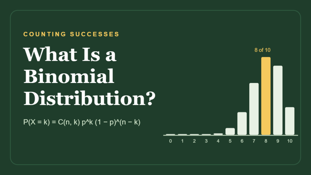
You plant 10 tomato seeds from a packet that says 80% of seeds sprout. How many seedlings should you expect? Probably 8, but 7 or 9 wouldn’t surprise you, and 4 would. A binomial probability distribution tells you exactly how likely each of those results is.
It is one of the most useful tools in statistics because so many everyday questions come down to “yes or no, repeated a set number of times.” Did the seed sprout? Did the customer click? Is the newborn a boy? Count the yeses and the binomial distribution describes the odds.
This guide explains what the binomial distribution is, the four conditions it needs, the formula in plain words, a full worked example, a real example using U.S. birth data, and the mistakes that trip people up.
Quick Info
| Topic | Detail |
|---|---|
| Short definition | The probability of getting exactly k successes in n independent yes/no trials |
| Key formula | P(X = k) = C(n, k) × p^k × (1 − p)^(n − k) |
| Conditions | Fixed number of trials, two outcomes, independent trials, same p each time |
| Mean and SD | Mean = np, SD = √(np(1 − p)) |
| Type | Discrete (only whole-number counts) |
| Common mistake | Using it when trials aren’t independent or p changes |
| Reading time | About 11 minutes |
What Is a Binomial Distribution?
A binomial distribution gives the probability of each possible number of successes when you repeat the same yes/no trial a fixed number of times, with the same chance of success every time.
“Success” doesn’t have to mean something good. It’s simply the outcome you’re counting. If you count defective light bulbs, a defective bulb is a “success.”
The word binomial means “two names,” a nod to the two possible outcomes of each trial. The result you care about, called X, is a count: 0, 1, 2 and so on up to n. Because X can only be a whole number, the binomial is a discrete distribution, and it’s usually drawn as a bar chart, much like a histogram.
The 4 Conditions for a Binomial Setting
Penn State’s online statistics course lists the conditions a situation must meet before the binomial model applies. In plain words:
Penn State STAT 414: The Binomial Distribution
| Condition | What it means | Seed example |
|---|---|---|
| Fixed number of trials (n) | You decide how many tries before you start | Exactly 10 seeds |
| Two outcomes | Each trial is success or failure | Sprouts or doesn’t |
| Independent trials | One result doesn’t change another | One seed doesn’t affect the next |
| Same probability (p) | The chance of success never changes | 80% for every seed |
Many teachers shorten this to BINS: Binary outcomes, Independent trials, Number of trials fixed, Same probability. If any letter fails, the binomial answer can be badly wrong.
Situations that are not binomial
- Flipping until you get heads. The number of trials isn’t fixed, so it’s a different model (the geometric distribution).
- Drawing cards without putting them back. Each draw changes the odds for the next one, so trials aren’t independent.
- Rolling a die and recording the number. There are six outcomes, not two, unless you redefine success as “rolled a six.”
The Binomial Formula, Explained
P(X = k) = C(n, k) × p^k × (1 − p)^(n − k)
- n is the number of trials.
- k is the number of successes you’re asking about.
- p is the chance of success on one trial, and 1 − p is the chance of failure.
- C(n, k), read “n choose k,” counts how many different orders could produce k successes.
C(n, k) = n! ÷ (k! × (n − k)!)
The ! means factorial: 5! = 5 × 4 × 3 × 2 × 1 = 120.
Why the formula has three parts
Think of one specific order, such as eight sprouts followed by two failures. Its probability is p multiplied eight times and (1 − p) multiplied twice: that’s p^k × (1 − p)^(n − k). But the two failures could be any two of the ten seeds, so you multiply by the number of possible orders, C(10, 8) = 45. Every order is equally likely, so adding them up is just multiplication.
Worked Example: 10 Tomato Seeds
A seed packet promises an 80% germination rate. You plant 10 seeds. What’s the chance that exactly 8 sprout? The figures are illustrative.
Step 1: Check the conditions
Ten seeds (fixed n), sprout or not (two outcomes), separate seeds (independent), 80% each (same p). The binomial model fits.
Step 2: Write down n, k and p
n = 10, k = 8, p = 0.8, 1 − p = 0.2
Step 3: Count the orders
C(10, 8) = 10! ÷ (8! × 2!) = 45
Step 4: Find the probability of one order
0.8^8 × 0.2^2 = 0.16777 × 0.04 = 0.006711
Step 5: Multiply
P(X = 8) = 45 × 0.006711 ≈ 0.302
There’s about a 30.2% chance that exactly 8 seeds sprout.
Step 6: Answer “at least” questions
Often you want a range, such as “at least 8 seedlings.” Add the probabilities for 8, 9 and 10:
| Seeds that sprout (k) | P(X = k) |
|---|---|
| 5 or fewer | 0.033 |
| 6 | 0.088 |
| 7 | 0.201 |
| 8 | 0.302 |
| 9 | 0.268 |
| 10 | 0.107 |
P(X ≥ 8) = 0.302 + 0.268 + 0.107 ≈ 0.678
So roughly two out of three gardeners planting 10 of these seeds will get 8 or more seedlings. About 1 in 30 will get 5 or fewer, which might be a sign that the packet’s 80% claim is too generous.
Try It: Build Your Own Binomial Distribution
Move the sliders to change the number of trials and the chance of success. The highlighted bar shows the count you pick, and the panel shows the probability of exactly that many, at most that many and at least that many successes.
Starts with the seed example: 10 seeds, 80% sprout rate. The dashed line marks the mean, n × p.
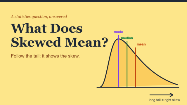
Notice what happens as you move p away from 0.5: the bars pile up on one side and a tail stretches toward the other. That’s a skewed distribution. At p = 0.5 the shape is perfectly symmetric.
Mean and Standard Deviation of a Binomial Distribution
You don’t need to list every probability to find the center and spread. Two short formulas do it:
Mean (expected value) = n × p
Standard deviation    = √(n × p × (1 − p))
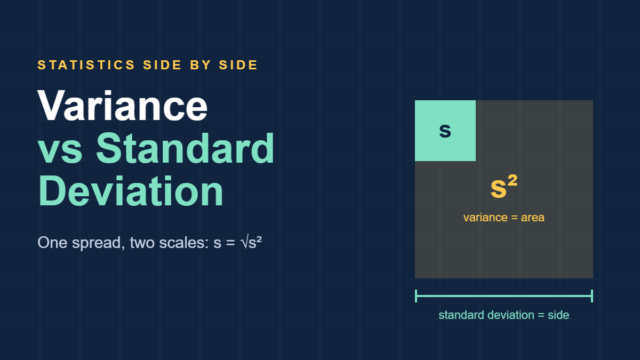
For the seeds, the mean is 10 × 0.8 = 8 seedlings, and the standard deviation is √(10 × 0.8 × 0.2) = √1.6 ≈ 1.26 seedlings. The variance is simply 1.6, the number under the square root.
The variance is largest when p = 0.5. A coin flip is as unpredictable as a yes/no trial can get, while a trial that almost always succeeds (p = 0.99) barely varies at all.
A Real Example: Boys and Girls in a Family of Four
Births give a real-world binomial setting. Slightly more boys are born than girls. The CDC’s National Center for Health Statistics reported a high of 1,059 boys per 1,000 girls born in 1946 and a low of 1,046 in 1991 and 2001.
CDC NCHS: More Boys Born Than Girls
Using about 1,050 boys per 1,000 girls, the chance that a baby is a boy is 1,050 ÷ 2,050 ≈ 0.512. Treat each birth in a family of four children as an independent trial (an approximation, since twins and family patterns exist):
| Outcome | Calculation | Probability |
|---|---|---|
| 2 boys and 2 girls | C(4, 2) × 0.512² × 0.488² | About 37.5% |
| All 4 boys | 0.512⁴ | About 6.9% |
| All 4 girls | 0.488⁴ | About 5.7% |
| All the same sex | 6.9% + 5.7% | About 12.5% |
Even the “most likely” result, an even split, happens in fewer than 4 out of 10 such families. That surprises a lot of people, and it’s a nice reminder that the expected value (about 2 boys) isn’t the same thing as a sure thing.
Binomial vs Normal Distribution
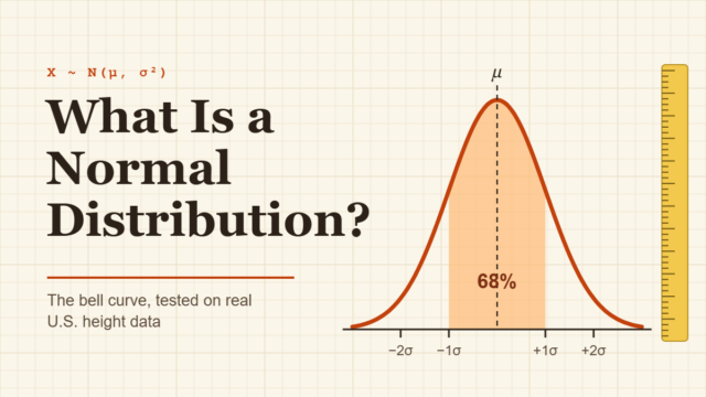
When n is large, the bars of a binomial distribution start to trace a smooth bell curve. Statisticians often use the normal distribution and z-scores as a shortcut when a common rule of thumb holds: both n × p and n × (1 − p) are at least 10.
| Feature | Binomial | Normal |
|---|---|---|
| Values | Whole-number counts | Any value on a continuous scale |
| Shape | Can be skewed | Always symmetric |
| Parameters | n and p | Mean and standard deviation |
| Best for | Counting successes | Measurements, or large-n approximations |
Real-Life Uses of the Binomial Distribution
- Quality control: the number of faulty items in a batch of 50, when each has a 2% defect rate.
- Medicine: how many of 20 patients respond to a treatment with a known response rate.
- Surveys: how many of 100 people in a random sample answer “yes.”
- Sports: a 75% free-throw shooter making at least 8 of 10 shots.
- Online marketing: clicks out of 1,000 emails sent, when 3% usually click.
Common Mistakes and Myths
| Myth | Reality |
|---|---|
| “The expected value is the most likely to happen every time.” | It’s the long-run average. In the family example, an even split happens only about 37% of the time. |
| “Any repeated experiment is binomial.” | Only if all four conditions hold, including a fixed n and the same p. |
| “Drawing without replacement is fine.” | It breaks independence. Use the hypergeometric model unless the population is huge. |
| “P(at least 1) = n × p.” | Use 1 − P(none) = 1 − (1 − p)^n instead. |
| “A binomial distribution is always symmetric.” | Only when p = 0.5. Otherwise it’s skewed. |
Frequently Asked Questions
What are the 4 conditions of a binomial distribution?
A fixed number of trials, only two possible outcomes per trial, independent trials, and the same probability of success on every trial. If even one of these fails, the binomial formula won’t give accurate probabilities, and another model, such as the geometric or hypergeometric distribution, may fit better.
What is the difference between binomial and Bernoulli?
A Bernoulli trial is a single yes/no experiment, like one coin flip. A binomial distribution counts the successes across several identical Bernoulli trials. So a binomial with n = 1 is just a Bernoulli trial, and a binomial with n = 10 adds up ten of them.
How do you calculate “at least” binomial probabilities?
Add the probabilities of every count in the range, or use the complement. For example, P(at least 1) equals 1 minus P(0). For “at least 8 out of 10,” add P(8), P(9) and P(10). The complement step (“not”) is one of the options in our Probability Calculator.
What is n choose k?
It’s the number of different ways to pick k items from n, ignoring order, written C(n, k) or nCk. In the binomial formula it counts how many different orders of successes and failures give exactly k successes. For example, C(10, 8) = 45.
Can you use a binomial distribution for a coin flip?
Yes. Each flip has two outcomes, flips are independent and the probability of heads stays at 0.5. The number of heads in, say, 20 flips follows a binomial distribution with n = 20 and p = 0.5. You can watch it in action with our Flip a Coin tool.
When should you use the normal approximation?
When n is large enough that both n × p and n × (1 − p) are at least 10, a common rule of thumb. Then the binomial bars look close to a bell curve, and normal probabilities give a good estimate with far less arithmetic.
Conclusion
The binomial distribution answers a simple but powerful question: if a yes/no event happens with the same probability each time, how likely is each possible count of successes? Check the four conditions first, then use C(n, k) × p^k × (1 − p)^(n − k) for exact probabilities, n × p for the expected count and √(np(1 − p)) for the spread.
A handy rule to remember: count the yeses, check the BINS. If the trials are binary, independent, fixed in number and share the same chance, the binomial distribution has your answer.
References
- Penn State Eberly College of Science, “STAT 414: The Binomial Distribution,” online.stat.psu.edu
- CDC National Center for Health Statistics, “More Boys Born Than Girls,” 2005, cdc.gov
Disclaimer
This article is for general educational purposes only. The seed germination figures in the worked example are illustrative. For research or professional analysis, consult a qualified statistician.