

You ask 30 coworkers how long their morning commute takes. You write down every answer: 12 minutes, 25, 34, 18, 41, and so on. By the end, you have a column of 30 numbers. The information is accurate, but it is difficult to understand the overall pattern at a glance.
Quick Info
| Topic | Detail |
|---|---|
| What it is | A chart that shows how numerical data is distributed using adjoining bars |
| X-axis | Data values divided into ranges called bins or classes |
| Y-axis | Frequency, relative frequency, or frequency density |
| Key feature | Adjacent bins are shown in order, with no gaps between their intervals |
| Built from | A grouped frequency distribution |
| Shows | Shape, centre, spread, gaps, and possible outliers |
| Reading time | About 10 minutes |
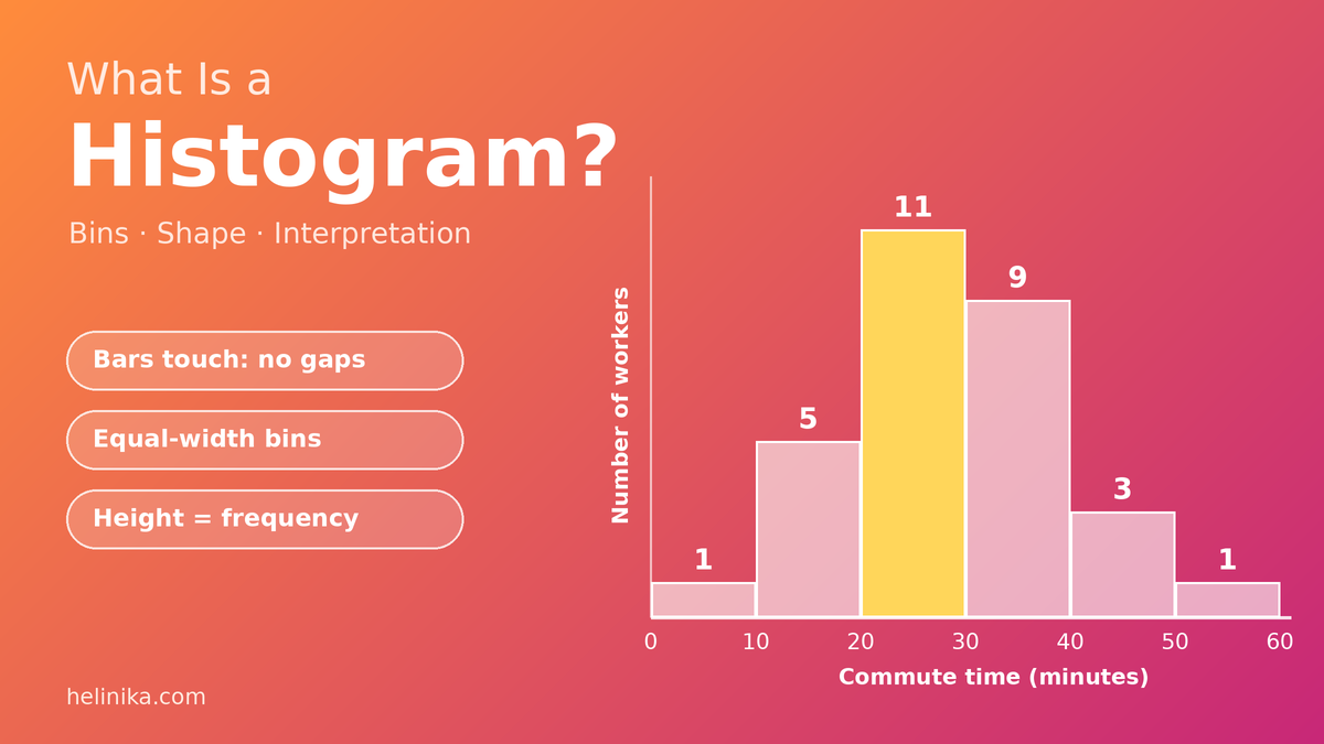
Now turn that list into a histogram. Suddenly, you can see that most people take between 20 and 40 minutes, one person takes less than 10 minutes, and another needs more than 50 minutes.
That’s the purpose of a histogram: to turn a collection of numerical values into a visual picture of how the data is distributed.
In this guide, you’ll learn what a histogram is, how bins work, how to create one step by step, and how to interpret the patterns it reveals.
What Is a Histogram?
A histogram is a chart that shows how numerical data is distributed across different ranges of values. These ranges are called bins or class intervals.
Each bar represents one bin, and its height shows how many observations fall within that range when the histogram displays frequency.
The bars are placed next to one another because the numerical intervals follow a continuous order. This is one of the main features that distinguishes a histogram from a standard bar chart.
The Statista statistics glossary also describes a histogram as a visual representation of a frequency distribution, with the measured variable on the horizontal axis and frequency on the vertical axis.
Histograms as a Data Visualization Tool
A list of numbers must be read one value at a time. A histogram allows you to see the overall distribution much faster.
It can help you identify:
- Where most observations are concentrated.
- Whether values are spread out or closely grouped.
- Whether the distribution is symmetrical or skewed.
- Whether there are gaps or unusual values.
- Whether the data appears to contain more than one group.
Histograms are commonly used in education, research, business, healthcare, and manufacturing to explore numerical data.
The Parts of a Histogram
A histogram contains several basic components:
| Part | What It Shows |
|---|---|
| Title | Describes what the data represents |
| X-axis (horizontal) | The numerical variable divided into bins |
| Y-axis (vertical) | Frequency, relative frequency, or frequency density |
| Bars | Represent the bins and their frequencies or densities |
| Axis labels and units | Explain the measurements, such as commute time in minutes |
For example, a histogram showing commute times might have “Commute Time (Minutes)” on the x-axis and “Number of Workers” on the y-axis.
Histogram vs. Bar Chart
Histograms and bar charts look similar because both use rectangular bars. However, they are designed for different types of information.
| Feature | Histogram | Bar Chart |
|---|---|---|
| Data type | Numerical data grouped into intervals | Categories or individual discrete values |
| X-axis | Numerical ranges or bins | Separate categories |
| Gaps between bars | Usually no gaps between adjacent intervals | Usually gaps between bars |
| Bar order | Follows numerical order | Can often be rearranged |
| Main purpose | Shows the distribution of numerical data | Compares categories or values |
| Example | Student heights in 5 cm groups | Students’ favourite sports |
A simple way to remember the difference is this: a histogram shows how numerical observations are distributed across ranges, while a bar chart compares separate categories.
What Are Bins in a Histogram?
A bin, also called a class or class interval, is a range into which numerical data is divided. Each bar in a histogram represents one bin.
For example, commute times might be divided into these intervals:
- 0–10 minutes
- 10–20 minutes
- 20–30 minutes
- 30–40 minutes
A commute lasting 25 minutes belongs in the 20–30 minute interval.
The NIST/SEMATECH e-Handbook of Statistical Methods explains the common approach of dividing a data range into bins and counting the observations that fall into each one.
Choosing the Bin Width
Bin width is an important decision when creating a histogram. The same data can look different depending on how wide or narrow the intervals are.
| Bin Selection | What Happens | Possible Result |
|---|---|---|
| Too few, very wide bins | Many values are combined | Important patterns may be hidden |
| Suitable bin width | The distribution is easier to see | Peaks, tails, and gaps become clearer |
| Too many, very narrow bins | Each bin contains very few values | The histogram may look noisy |
A practical method for choosing bin width is:
- Find the range by subtracting the lowest value from the highest value.
- Choose a reasonable number of bins. Five to ten can be a useful starting point for a small classroom data set.
- Divide the range by the number of bins.
- Round the result up to a convenient width, such as 5, 10, or 20.
Formula:
Bin width ≈ (Highest value − Lowest value) ÷ Number of bins
For larger data sets, you may need more bins. Statistical methods such as Sturges’ rule and Scott’s rule can also help determine a suitable bin width.
The best choice depends on the amount of data and the level of detail you want to show.
The Boundary Rule
What happens when a value falls exactly on the boundary between two bins?
For example, where should a commute time of 20 minutes go if the intervals are 10–20 and 20–30?
A common convention is to include the lower boundary but exclude the upper boundary. Under this rule:
- The 10–20 bin includes 10 but excludes 20.
- The 20–30 bin includes 20 but excludes 30.
Therefore, a value of 20 belongs in the 20–30 bin.
Whatever convention you choose, every observation must belong to exactly one bin.
Why Equal Bin Widths Matter
Equal-width bins make histograms easier to read and compare. When all intervals have the same width, bar height can represent frequency directly.
However, some histograms use unequal bin widths. In those cases, bar height should represent frequency density, not simply frequency.
Frequency density = Frequency ÷ Bin width
The area of each bar then represents its frequency. This prevents wider intervals from appearing more important simply because they cover a larger numerical range.
How to Draw a Histogram: Worked Example
Let’s create a histogram using the morning commute times, in minutes, of 30 office workers:
12, 25, 34, 18, 41, 27, 22, 38, 15, 29, 33, 47, 21, 26, 31, 8, 36, 24, 28, 52, 19, 35, 30, 23, 44, 27, 32, 16, 39, 26
Step 1: Find the Range
Identify the lowest and highest values:
- Lowest value = 8
- Highest value = 52
Subtract the lowest value from the highest:
Range = 52 − 8 = 44 minutes
Step 2: Choose the Bins
We’ll use approximately six bins.
44 ÷ 6 ≈ 7.3
Rounding up to a convenient width of 10 minutes gives us these intervals:
0–10, 10–20, 20–30, 30–40, 40–50, and 50–60.
Starting at zero makes the intervals straightforward and ensures that every observation is included.
Step 3: Build the Frequency Table
Count how many commute times fall into each interval, including the lower boundary but excluding the upper boundary.
| Commute Time (Minutes) | Frequency |
|---|---|
| 0–10 | 1 |
| 10–20 | 5 |
| 20–30 | 11 |
| 30–40 | 9 |
| 40–50 | 3 |
| 50–60 | 1 |
| Total | 30 |
The frequencies add up to 30, matching the number of workers in the original data set.
This is a grouped frequency distribution table, which provides the information needed to draw the histogram. If you want to learn more about organizing data this way, read our guide to frequency distribution tables.
Step 4: Draw the Axes
Set up the horizontal and vertical axes:
- X-axis: Label it “Commute Time (Minutes)” and mark 0, 10, 20, 30, 40, 50, and 60.
- Y-axis: Label it “Number of Workers” and use a scale that reaches at least 12.
Step 5: Draw the Bars
Draw one bar for each interval. Its height should match the frequency in the table.
For example:
- The 0–10 bin has a height of 1.
- The 20–30 bin has a height of 11.
- The 30–40 bin has a height of 9.
- The 50–60 bin has a height of 1.
The bars should be adjacent, with no spaces between their intervals.
Step 6: Add a Title and Labels
Give the chart a clear title, such as:
“Morning Commute Times of 30 Office Workers”
Make sure both axes have labels and the measurement units are included.
What Happens With Narrower Bins?
Let’s use the same commute data but divide it into 5-minute intervals instead of 10-minute intervals.
| Commute Time (Minutes) | Frequency |
|---|---|
| 5–10 | 1 |
| 10–15 | 1 |
| 15–20 | 4 |
| 20–25 | 4 |
| 25–30 | 7 |
| 30–35 | 5 |
| 35–40 | 4 |
| 40–45 | 2 |
| 45–50 | 1 |
| 50–55 | 1 |
| Total | 30 |
The overall concentration in the middle is still visible, but the distribution looks more detailed and slightly bumpier.
With only 30 observations, 10-minute intervals provide a simpler overview. With a larger data set, narrower intervals may reveal additional patterns.
How to Interpret a Histogram
Drawing a histogram is only the first step. The real value comes from understanding what its shape and bars tell you.
When interpreting a histogram, consider four things: shape, centre, spread, and unusual values.
1. Look at the Shape
The overall shape can reveal how observations are distributed.
| Shape | What It Looks Like | What It Often Means | Example |
|---|---|---|---|
| Symmetric | Both sides look roughly similar | Values are concentrated around the centre | Some adult height distributions |
| Right-skewed | A long tail extends to the right | Most values are relatively low, with a few high values | Household income |
| Left-skewed | A long tail extends to the left | Most values are relatively high, with a few low values | Scores on some easy tests |
| Bimodal | Two noticeable peaks | The data may contain two different groups | Commute times for two work shifts |
| Uniform | Bars have roughly similar heights | Values occur at fairly similar frequencies | Results from many rolls of a fair die |
The NIST handbook describes the classical bell-shaped histogram as having most observations near the centre, with fewer values toward the tails.
A useful way to remember skewness is that the tail points in the direction of the skew. A long tail extending to the right indicates a right-skewed distribution.
2. Find the Centre
The tallest bar identifies the modal class, which is the interval containing the greatest number of observations.
In our commute example, the modal class is 20–30 minutes because it contains 11 workers.
The distribution’s shape can also provide clues about the relationship between the mean and median:
- Symmetric distribution: The mean and median are often close.
- Right-skewed distribution: The mean is often greater than the median because high values pull it toward the right.
- Left-skewed distribution: The mean is often smaller than the median because low values pull it toward the left.
For our commute data, the mean is:
858 ÷ 30 = 28.6 minutes
The median is 27.5 minutes.
The mean and median are relatively close, which is consistent with the data being roughly balanced, although the distribution is not perfectly symmetric.
For a more detailed explanation of averages, see our guide on what a mean is in statistics.
3. Judge the Spread
The spread describes how widely the observations are distributed.
- A narrow histogram suggests that values are concentrated within a smaller range.
- A wider histogram suggests that observations cover a larger range.
In the commute example, times extend from 8 to 52 minutes. However, 20 of the 30 workers have commutes between 20 and 40 minutes.
This tells us that most observations are concentrated in the middle, even though the overall range is wider.
4. Spot Gaps and Outliers
Look for empty intervals or isolated bars that are separated from the main group of observations.
An empty bin may indicate a gap in the data or suggest that observations come from different groups.
An isolated value may be an outlier, but a histogram alone cannot confirm that it is an error or an unusual measurement. It should be investigated using the original data and other relevant information.
Reading Bar Area
For equal-width bins, bar height represents frequency, so comparing heights is straightforward.
However, when bins have unequal widths, the area of each bar represents frequency rather than height alone.
This is because:
Bar area = Bin width × Bar height
In an unequal-width histogram, the height is usually calculated using frequency density:
Frequency density = Frequency ÷ Bin width
This distinction matters because a wider interval may contain more observations simply because it covers a larger range. Using frequency density keeps the comparison fair.
Where Histograms Are Used in Real Life
Histograms are useful in many areas:
- Education: Showing how exam marks are distributed across a class.
- Healthcare: Studying distributions of measurements such as blood pressure or weight.
- Weather: Displaying how often different rainfall amounts occur.
- Business: Analyzing customer ages, order values, or delivery times.
- Manufacturing: Checking whether product measurements remain within acceptable limits.
- Photography: A camera histogram displays how image pixels are distributed across brightness levels, from dark to bright.
These examples show how histograms help people understand numerical patterns without examining every individual observation.
Common Mistakes to Avoid
When creating or interpreting a histogram, watch out for these common errors:
- Leaving gaps between adjacent intervals: Histogram intervals should be continuous, and their bars are normally drawn next to each other.
- Using unequal bin widths without adjustment: For unequal-width bins, use frequency density so bar area represents frequency.
- Choosing unsuitable bin widths: Too few or too many bins can hide important patterns.
- Overlapping intervals: A value on a boundary must belong to exactly one bin.
- Using a histogram for unordered categories: Favourite colours and subjects are generally better displayed with a bar chart.
- Forgetting axis labels and units: Without labels, readers may not understand what the chart represents.
- Assuming every unusual bar is an outlier: Check the original observations before drawing conclusions.
Frequently Asked Questions
What is a histogram in simple words?
A histogram is a chart with adjoining bars that shows how many numerical observations fall within different ranges.
What are bins in a histogram?
Bins are the ranges into which numerical data is divided. For example, a histogram of commute times might use intervals such as 0–10, 10–20, and 20–30 minutes.
Why do histogram bars touch?
Histogram bars represent adjacent numerical intervals. Since one interval follows directly after another, the bars are normally drawn without gaps.
How many bins should a histogram have?
Five to ten bins can be a useful starting point for many small data sets. Larger data sets may need more bins. The best number depends on the amount and distribution of the data.
What does a skewed histogram mean?
A skewed histogram has a longer tail on one side than the other. A right-skewed distribution has a tail extending to the right, while a left-skewed distribution has a tail extending to the left.
Can a histogram show percentages instead of counts?
Yes. A relative frequency histogram shows the proportion or percentage of observations in each bin instead of the raw count. For unequal-width bins, the bar height must be adjusted so that bar area represents the relative frequency.
Conclusion
A histogram turns a list of numerical observations into a visual representation of how data is distributed. Divide the values into suitable bins, count the observations in each interval, and draw adjoining bars to display the results.
The most useful skill is learning how to interpret the chart. Look at its shape, identify the centre, judge the spread, and investigate any unusual patterns.
With practice, a histogram can reveal important information about a data set much faster than a long list of numbers.
References
Disclaimer
This article is for general educational purposes only. The examples use simplified data to explain how histograms work. Bin selection, boundary conventions, and histogram scales may vary depending on the data and the requirements of a textbook or exam board. Follow your teacher’s or syllabus guidelines when completing academic work.