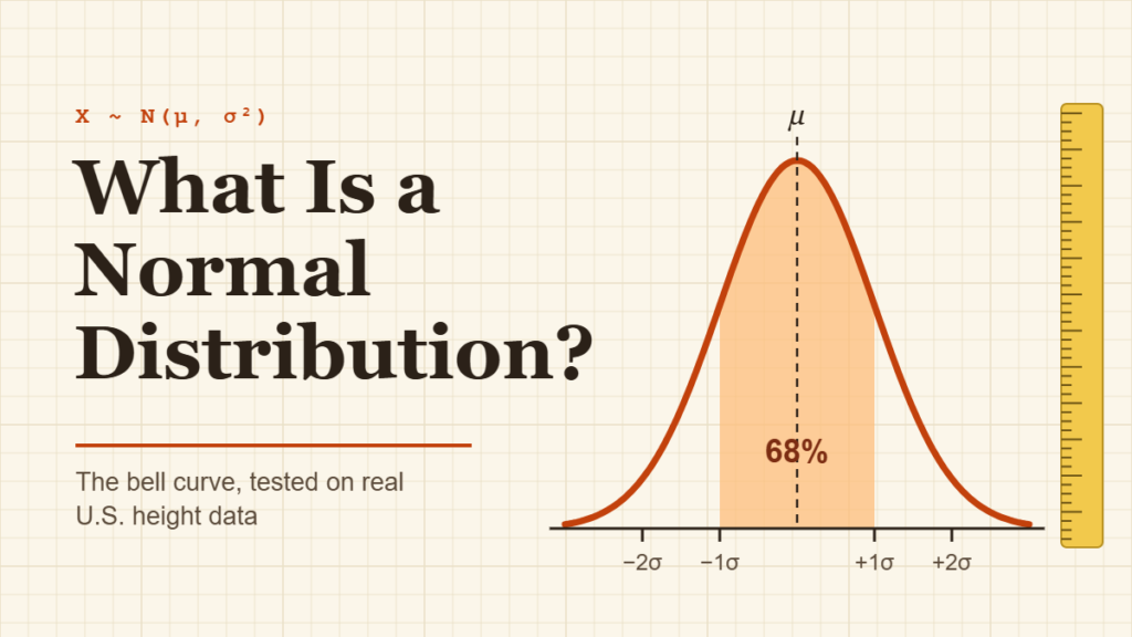
Line up 100 American women by height and something neat happens. Most of them crowd around 5 feet 3 or 4 inches, fewer stand at 5 feet or 5 feet 7, and only a handful sit at the far ends. Sketch that crowd as a curve and you get a smooth hill with matching slopes on each side: the normal distribution bell curve.
It’s the most famous shape in statistics, and for good reason. Once you know a set of data is roughly normal, two numbers (the mean and the standard deviation) tell you almost everything about it, including how rare any single value is.
This guide explains what a normal distribution is, the properties that define it, a worked example, and a real test: we check the bell curve against height data measured by the CDC on more than 10,000 U.S. adults. You’ll also see when data is not normal and how to spot it.
Quick Info
| Topic | Detail |
|---|---|
| Short definition | A symmetric, bell-shaped distribution set entirely by its mean and standard deviation |
| Notation | X ~ N(μ, σ²) |
| Center | Mean = median = mode, all at the peak |
| Key conversion | z = (x − μ) ÷ σ turns any normal value into a standard normal value |
| Real example | Adult height in the U.S. is close to normal within each sex |
| Common mistake | Assuming income, wait times or house prices are normal (they’re skewed) |
| Reading time | About 11 minutes |
What Is a Normal Distribution?
A normal distribution is a continuous probability distribution that is symmetric around its mean, highest at the center, and tapers off evenly on both sides, forming a bell shape.
It’s also called the Gaussian distribution, after mathematician Carl Friedrich Gauss. “Bell curve” is the everyday name, and it describes the picture well: a rounded top with long, thin tails.
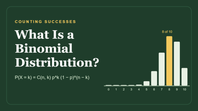
The distribution is continuous, which means a value can land anywhere on the number line, not just on whole numbers. That’s the opposite of a count like “number of heads in 10 flips,” which follows a binomial distribution and is drawn as separate bars.
Because the curve is continuous, you never ask “what’s the chance of exactly 64 inches?” (the answer is zero). You ask about ranges instead: “what share of women are between 62 and 66 inches?” That share is the area under the curve over that range.
The 6 Properties of a Normal Distribution
Penn State’s probability course sets out the core facts about every normal curve: it’s bell-shaped, symmetric about the mean, highest at the mean, and the total area under it equals 1.
Penn State STAT 414: Normal Distributions
Here are those facts in plain words, plus two practical ones:
| Property | What it means for you |
|---|---|
| Bell-shaped | One peak, no gaps, smooth slopes |
| Symmetric | The left half is a mirror image of the right half |
| Mean = median = mode | The average, the middle value and the most common value sit at the same point |
| Total area = 1 | All the probabilities add up to 100% |
| Set by two numbers | The mean fixes where the peak sits; the standard deviation fixes how wide it spreads |
| Tails never touch zero | Extreme values are rare, but never strictly impossible |
How the mean and standard deviation change the curve
Think of the mean as a slider that moves the whole bell left or right without changing its shape. The standard deviation works like a zoom: a small SD gives a tall, narrow bell, and a large SD gives a short, wide one. The area always stays at 1, so when the bell gets wider it has to get flatter.
The inflection points
Look closely at a bell curve and you’ll see the slope switch from “curving down” to “curving up” at two spots. Those spots sit exactly one standard deviation either side of the mean. It’s a handy way to eyeball the SD straight off a graph.
The Normal Distribution Formula
You’ll rarely calculate it by hand, but here is the formula for the height of the curve at any value x:
f(x) = (1 ÷ (σ√(2π))) × e^(−(x − μ)² ÷ (2σ²))
- x is the value you’re looking at (for example, a height of 66 inches).
- μ (mu) is the mean of the distribution.
- σ (sigma) is the standard deviation.
- e and π are fixed constants, about 2.718 and 3.142.
The important part is the (x − μ)² in the exponent. The farther x sits from the mean, the bigger that term gets and the faster the curve drops. Squaring it also makes the drop identical on both sides, which is why the curve is symmetric.
The Standard Normal Distribution and Z-Scores
Every normal distribution has its own mean and SD, so tables and calculators use one reference version: the standard normal distribution, with a mean of 0 and a standard deviation of 1.
You move any value onto that standard scale with a z-score:
z = (x − μ) ÷ σ
A z-score tells you how many standard deviations a value sits above or below the mean. Once you have z, the area to its left gives the share of values below it. That’s how a bell curve turns a raw measurement into a percentile.
You may already know the 68-95-99.7 rule: about 68% of values fall within 1 SD of the mean, 95% within 2 SDs and 99.7% within 3. We cover it step by step in our standard deviation guide, so here we’ll put the curve to work instead.
Worked Example: How Rare Is a 6-Foot Man?
Let’s answer a question people actually wonder about: what share of American men are shorter than 6 feet?
Step 1: Get the mean and standard deviation
The CDC’s National Center for Health Statistics measured 5,092 men aged 20 and over in its 2015–2018 health survey. Their mean height was 69.0 inches (5 feet 9 inches).
CDC NCHS: Anthropometric Reference Data for Children and Adults, United States, 2015–2018
The report publishes percentiles rather than a standard deviation, so we estimated it from the spread between the 5th and 95th percentiles (64.1 and 73.8 inches). In a normal distribution those two points sit 1.645 SDs either side of the mean, which gives:
SD ≈ (73.8 − 64.1) ÷ (2 × 1.645) ≈ 2.9 inches
Step 2: Convert 6 feet to a z-score
Six feet is 72 inches.
z = (72 − 69.0) ÷ 2.9 ≈ 1.03
A 6-foot man is about one standard deviation above average.
Step 3: Find the area to the left
The standard normal area to the left of z = 1.03 is about 0.85. So roughly 85% of U.S. men are shorter than 6 feet, and about 15% are 6 feet or taller.
Step 4: Check it against the real data
Here’s the satisfying part. The CDC’s measured 85th percentile for men is 72.0 inches: exactly 6 feet. The bell curve, built from just two numbers, landed on the real answer.
Try It: Where Does a Height Fall on the Bell Curve?
Pick women or men, then drag the slider. The shaded area shows the share of adults shorter than the height you choose, and the orange markers show where the CDC’s real percentiles fall. Notice how closely the markers sit to where the curve says they should.
Shaded area = share of adults shorter than the chosen height. Orange ticks mark the real CDC percentiles (10th, 25th, 50th, 75th, 90th).
Real Test: Does U.S. Height Really Follow a Bell Curve?
One lucky match proves nothing, so let's test the whole curve. Using the means from the CDC report and the SDs estimated in the worked example (2.7 inches for women, 2.9 for men), we asked the normal distribution to predict seven percentiles, then compared them with what the CDC measured.
| Percentile | Women: CDC measured | Women: bell curve | Men: CDC measured | Men: bell curve |
|---|---|---|---|---|
| 5th | 59.0 in | 59.1 in | 64.1 in | 64.2 in |
| 10th | 60.0 in | 60.0 in | 65.3 in | 65.3 in |
| 25th | 61.6 in | 61.7 in | 67.0 in | 67.0 in |
| 50th | 63.5 in | 63.5 in | 69.1 in | 69.0 in |
| 75th | 65.3 in | 65.3 in | 71.0 in | 71.0 in |
| 90th | 67.0 in | 67.0 in | 72.7 in | 72.7 in |
| 95th | 67.9 in | 67.9 in | 73.8 in | 73.8 in |
Every prediction lands within 0.1 inch of the measured value. Two more clues point the same way. The women's mean (63.5) equals their median (63.5), and the men's mean (69.0) sits just 0.1 inch from their median (69.1). In a normal distribution, those two should match.
One honest caveat: this works because we split by sex. Pool men and women together and you're mixing two bells with peaks about 5.5 inches apart, which gives a wider, flatter hump that isn't a true normal curve.
Why So Many Things Follow a Bell Curve
Height is shaped by hundreds of small influences: many genes, childhood nutrition, health, sleep and more. Each one nudges a person a little taller or shorter, and the nudges mostly cancel out. When lots of small, independent effects add up, the total tends to form a bell. That's the idea behind the central limit theorem.
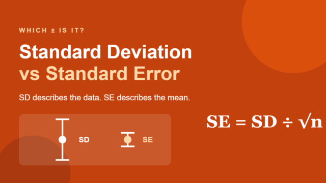
The same theorem explains why sample averages are close to normal even when the raw data isn't. Average 50 random wait times and repeat the process many times, and those averages will pile up in a bell around the true mean. Their spread is measured by the standard error, and it's the reason confidence intervals and many tests rely on the normal curve.
When Data Is Not Normal
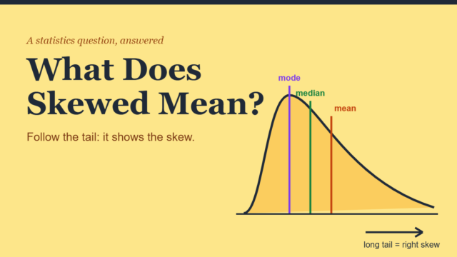
Plenty of real data refuses to form a bell. The usual culprit is a hard floor with no ceiling: a wait time can't drop below zero but can stretch to an hour, and pay can't go below zero but can run into the millions. That produces a long tail on one side, a shape called skewed.
| Usually close to normal | Usually not normal |
|---|---|
| Adult height (within one sex) | Household income and weekly pay (right-skewed) |
| Measurement errors on a lab scale | Time waiting in line or on hold (right-skewed) |
| Weights of bags filled by the same machine | House prices (right-skewed) |
| Averages of many repeated samples | Test scores on a very easy exam (left-skewed) |
| Blood pressure within a healthy group | Number of children in a family (counts, few values) |
3 quick ways to check for normality
- Draw a histogram. Look for one central peak and roughly matching sides. Two peaks, a long tail or a cliff at one end are warning signs.
- Compare the mean and the median. If they're far apart relative to the SD, the data is probably skewed.
- Test a few percentiles, like we did with height. If the 10th and 90th percentiles sit about 1.28 SDs from the mean, the bell is a decent fit.
With large datasets, statisticians also use a normal quantile plot (Q-Q plot), where normal data falls along a straight line.
Common Myths About the Bell Curve
| Myth | Reality |
|---|---|
| "Normal" means typical or healthy | It's just the name of a shape, not a judgment about people or data |
| Most data is normally distributed | Lots of data is skewed, lumpy or bounded; always check first |
| A bell-shaped histogram proves normality | It's a good sign, but tails and peaks can still differ from a true normal curve |
| You need a big sample for the curve to exist | The curve is a model of the population; a small sample just gives a rough picture of it |
| Grading on a curve makes scores normal | It forces grades into set shares; the actual scores can have any shape |
Frequently Asked Questions
Why is it called a bell curve?
Because the graph looks like the outline of a bell: tall and rounded in the middle, flaring out into thin edges on both sides. The name describes the picture, not a rule. Statisticians usually say "normal distribution" or "Gaussian distribution," and all three names mean the same shape.
What is the difference between a normal and a standard normal distribution?
A normal distribution can have any mean and any standard deviation, such as women's height with a mean of 63.5 inches and an SD of 2.7. The standard normal distribution is the single special case with a mean of 0 and an SD of 1. You convert between them with z = (x − μ) ÷ σ.
Is the normal distribution discrete or continuous?
Continuous. A normal variable can take any value within a range, including decimals, so you find probabilities as areas under the curve over an interval. Counts that can only be whole numbers, like the number of heads in a set of flips, are discrete and use distributions such as the binomial instead.
Is the mean always equal to the median in a normal distribution?
Yes. Because the curve is perfectly symmetric, the mean, median and mode all sit at the peak. Real data that's close to normal shows them close together too, as with U.S. women's height, where the CDC's mean and median are both 63.5 inches. A big gap between them usually signals skew.
Can a normal distribution have negative values?
In theory, yes: the tails stretch forever in both directions. In practice it often doesn't matter. For men's height, 0 inches sits more than 23 standard deviations below the mean, so the probability is too small to measure. When negative values are impossible and the data sits close to zero, a different model usually fits better.
What does it mean if my data is not normal?
Nothing is wrong with it. It just means methods built on the bell curve, like reading percentiles straight from z-scores, may give misleading answers. You can describe the data with the median and percentiles instead, transform it (taking logs often tames right skew), or use methods that don't assume normality.
Conclusion
A normal distribution is a symmetric bell built from just two numbers, the mean and the standard deviation. When data truly follows it, you can turn any value into a z-score and read off how common or rare it is, as we did when the curve correctly placed a 6-foot man at the 85th percentile of U.S. height. The bell is powerful, but it's a model, not a law of nature.
Before you trust the curve, ask one question: are lots of small, independent effects adding up here, or is there a floor that lets one tail run long?
Disclaimer
This article is for general educational purposes only. The standard deviations used for U.S. height are estimates derived from published CDC percentiles, and individual growth or health questions should go to a doctor. For research or business analysis, consult a qualified statistician.