

A teacher hands you a sheet with 30 test scores written in no particular order. You want to know how many students scored above 15. You would have to scan the list, count the scores, and probably check your answer again.
Quick Info
| Topic | Detail |
|---|---|
| What it is | A table showing how often each value or group of values occurs |
| Main columns | Value or class, tally, and frequency |
| Extra columns | Relative frequency, percentage, and cumulative frequency |
| Main types | Ungrouped and grouped frequency tables |
| Key check | All frequencies must add up to the total number of observations |
| Common uses | Organizing data, creating charts, and calculating mean, median, and mode |
| Reading time | About 9 minutes |
Now imagine those scores arranged in a table, with each value in one column and the number of times it appears in the next. The answer becomes much easier to find.
That table is called a frequency distribution table. It helps organize raw data so you can identify common values, compare groups, and understand patterns more quickly.
In this guide, you’ll learn what a frequency distribution table is, what its columns mean, and how to create ungrouped and grouped tables using step-by-step examples.
What Is a Frequency Distribution Table?
A frequency distribution table is a way of organizing data that shows each value, or group of values, alongside the number of times it appears. This count is called its frequency.
The table makes it easier to understand how data is distributed, including which values occur most often and which are less common.
Why Organizing Data Matters
Raw data is simply a list of collected values. Although the information is there, a long list can be difficult to read and interpret.
Organizing it into a frequency table offers several benefits:
- Shows patterns clearly: You can quickly identify common and rare values.
- Makes large data sets easier to read: Hundreds of observations can be summarized in a smaller table.
- Supports further analysis: Frequency tables can help you create charts and calculate statistics such as the mean, median, and mode.
For example, our guide on what a mean is in statistics explains how frequency information can help calculate an average when values repeat.
Raw Data vs. Organized Data
Suppose a teacher records the number of siblings reported by 20 students:
2, 1, 0, 3, 1, 2, 1, 1, 0, 2, 4, 1, 2, 0, 1, 3, 2, 1, 1, 2
This list is the raw data. We can organize it into a frequency distribution table:
| Number of siblings | Frequency |
|---|---|
| 0 | 3 |
| 1 | 8 |
| 2 | 6 |
| 3 | 2 |
| 4 | 1 |
| Total | 20 |
The table shows that having one sibling is the most common result, while having four siblings is the least common.
No observations have been removed. The information is simply easier to understand.
What Kind of Data Can Go in a Frequency Table?
Frequency tables can organize both qualitative and quantitative data.
- Qualitative data describes categories or qualities, such as eye colour, favourite subjects, or product types. These values are not numerical measurements.
- Quantitative data consists of numerical values, such as ages, test scores, heights, or temperatures.
Both types can be counted and displayed in a frequency table. However, calculations such as the mean are generally appropriate only for numerical data.
The Frequency Columns Explained
A basic frequency table needs two columns: the value or class and its frequency. You can also include additional columns to answer more detailed questions.
Here is the siblings data again, with the common frequency columns included:
| Siblings (x) | Tally | Frequency (f) | Relative frequency | Percentage | Cumulative frequency |
|---|---|---|---|---|---|
| 0 | III | 3 | 0.15 | 15% | 3 |
| 1 | IIII/ III | 8 | 0.40 | 40% | 11 |
| 2 | IIII/ I | 6 | 0.30 | 30% | 17 |
| 3 | II | 2 | 0.10 | 10% | 19 |
| 4 | I | 1 | 0.05 | 5% | 20 |
| Total | 20 | 1.00 | 100% | 20 |
In handwritten tally marks, the fifth mark crosses the previous four. This makes groups of five easier to count.
1. Value or Class Column
The first column identifies what you are counting.
In an ungrouped table, it lists individual values, such as 0, 1, 2, and 3.
In a grouped table, it lists class intervals, such as 10–20 or 20–30.
2. Tally Column
Tally marks help you count observations as you go through the raw data.
You make one mark for each value and group the marks in fives. This makes it easier to track your counting and reduces mistakes.
A tally column is optional in the final table, but it is useful when organizing data manually.
3. Frequency Column (f)
Frequency is the number of times a particular value or class appears.
For example, if eight students have one sibling, the frequency for one sibling is 8.
The sum of all frequencies must equal the total number of observations. If it does not, you may have missed or counted an observation more than once.
4. Relative Frequency Column
Relative frequency shows what proportion of the total observations belongs to a particular value or class.
Formula:
Relative frequency = Frequency ÷ Total frequency
For example, the relative frequency of students with one sibling is:
8 ÷ 20 = 0.40
Relative frequencies add up to 1 when calculated without rounding.
The NIST/SEMATECH e-Handbook of Statistical Methods uses the same basic idea when describing relative frequencies in histograms.
5. Percentage Column
A percentage expresses relative frequency out of 100.
Formula:
Percentage = Relative frequency × 100
For the students with one sibling:
0.40 × 100 = 40%
This means 40% of the students in the example have one sibling.
6. Cumulative Frequency Column
Cumulative frequency is a running total of the frequencies up to and including the current row.
For example:
- For 0 siblings, the cumulative frequency is 3.
- For 1 sibling, it is 3 + 8 = 11.
- For 2 siblings, it is 11 + 6 = 17.
This column answers questions such as, “How many students have two or fewer siblings?”
The final cumulative frequency should equal the total number of observations.
Cumulative frequency is most useful when values or classes have a natural order. It is generally not meaningful for unordered categories such as favourite colours.
How to Make a Frequency Distribution Table
There are two common ways to organize numerical data: an ungrouped frequency table and a grouped frequency table.
| Feature | Ungrouped table | Grouped table |
|---|---|---|
| Each row shows | One individual value | A range of values |
| Best for | Data with few distinct values | Data with many different values |
| Detail | Keeps exact values visible | Combines values into intervals |
| Example row | 3 siblings → frequency 2 | 20–30 kg → frequency 7 |
Steps for an Ungrouped Frequency Table
Follow these steps:
- List every distinct value in ascending order.
- Go through the raw data and make a tally mark beside each value.
- Count the tally marks and record the frequency.
- Add all frequencies and check that the total matches the number of observations.
- Add relative frequency, percentage, or cumulative frequency columns if needed.
Steps for a Grouped Frequency Table
When data contains many different values, creating a separate row for each value can make the table too long. Grouping values into class intervals makes the information easier to read.
Follow these steps:
- Find the range: Subtract the smallest value from the largest value.
- Choose the number of classes: Five to ten classes can be a useful starting point for many small classroom data sets, but the best number depends on the data and purpose.
- Calculate the class width: Divide the range by the number of classes and round up to a convenient width.
- Create the intervals: Start at or slightly below the smallest observation.
- Tally the values: Count how many observations fall into each interval.
- Check the total: Make sure all frequencies add up to the number of observations.
Formula:
Class width ≈ (Highest value − Lowest value) ÷ Number of classes
A Rule That Avoids Double Counting
A value on a class boundary must belong to exactly one interval.
A common convention is to include the lower limit but exclude the upper limit. Under this rule:
- 10–20 includes 10 but excludes 20.
- 20–30 includes 20 but excludes 30.
Therefore, a value of 20 belongs in the 20–30 class, not the 10–20 class.
Some textbooks use whole-number intervals such as 10–19 and 20–29 instead. Follow the convention required by your textbook or exam board.
Worked Examples
Example 1: Ungrouped Frequency Table (Shoe Sizes)
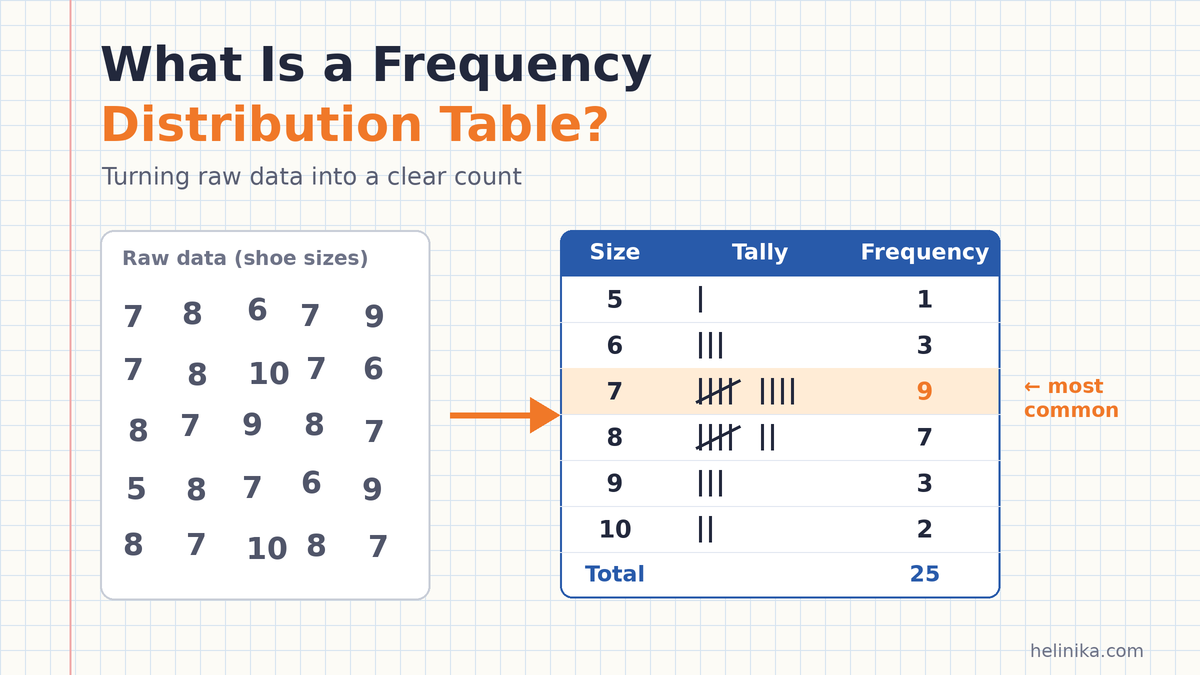
A shoe shop records the sizes purchased by 25 customers on a Saturday:
7, 8, 6, 7, 9, 7, 8, 10, 7, 6, 8, 7, 9, 8, 7, 5, 8, 7, 6, 9, 8, 7, 10, 8, 7
There are only six different shoe sizes, so an ungrouped table is suitable.
| Shoe size | Tally | Frequency (f) | Percentage | Cumulative frequency |
|---|---|---|---|---|
| 5 | I | 1 | 4% | 1 |
| 6 | III | 3 | 12% | 4 |
| 7 | IIII/ IIII | 9 | 36% | 13 |
| 8 | IIII/ II | 7 | 28% | 20 |
| 9 | III | 3 | 12% | 23 |
| 10 | II | 2 | 8% | 25 |
| Total | 25 | 100% | 25 |
What does the table tell the shop owner?
- Size 7 is the best seller, with 9 purchases or 36% of the total.
- Sizes 7 and 8 together account for 16 purchases, or 64%.
- Five customers purchased size 9 or larger, representing 20% of sales.
Example 2: Grouped Frequency Table (Test Marks)
Thirty students take a test marked out of 50. Their scores are:
23, 41, 35, 18, 29, 44, 31, 27, 38, 12, 33, 26, 47, 30, 21, 36, 40, 28, 15, 34, 25, 39, 32, 9, 43, 37, 29, 24, 35, 31
There are many different scores, so grouping them into class intervals makes the data easier to summarize.
First, calculate the range:
47 − 9 = 38
Next, choose five classes. The approximate class width is:
38 ÷ 5 = 7.6
Rounding up to a convenient width of 10 gives these intervals:
0–10, 10–20, 20–30, 30–40, and 40–50.
Using the lower-inclusive, upper-exclusive convention, the completed table is:
| Marks | Frequency (f) | Relative frequency | Cumulative frequency |
|---|---|---|---|
| 0–10 | 1 | 0.03 | 1 |
| 10–20 | 3 | 0.10 | 4 |
| 20–30 | 9 | 0.30 | 13 |
| 30–40 | 12 | 0.40 | 25 |
| 40–50 | 5 | 0.17 | 30 |
| Total | 30 | 1.00 | 30 |
Relative frequencies are rounded to two decimal places.
Notice that a score of 30 belongs in the 30–40 class, not the 20–30 class. The table shows that most students scored between 30 and 40, while 13 students scored below 30.
Example 3: Categorical Data (Favourite Subjects)
A class of 30 students is asked to name their favourite subject. Because the answers are categories rather than numerical measurements, this is qualitative data.
| Favourite subject | Frequency (f) | Percentage |
|---|---|---|
| Maths | 9 | 30% |
| Science | 8 | 26.67% |
| English | 6 | 20% |
| Urdu | 4 | 13.33% |
| Art | 3 | 10% |
| Total | 30 | 100% |
The table shows that Maths is the most popular subject, selected by 30% of the class.
For unordered categories, sorting the rows from most popular to least popular can make comparisons easier. Cumulative frequency is usually left out because these categories have no natural numerical order.
Example 4: Angles From a Geometry Worksheet
A student measures 20 angles on a geometry worksheet:
35°, 120°, 90°, 62°, 145°, 88°, 90°, 170°, 45°, 110°, 73°, 90°, 155°, 28°, 95°, 60°, 130°, 90°, 15°, 100°
The same observations can be organized in different ways, depending on the question being asked.
Organized by angle type:
| Angle type | Frequency |
|---|---|
| Acute (less than 90°) | 8 |
| Right (exactly 90°) | 4 |
| Obtuse (greater than 90° and less than 180°) | 8 |
| Total | 20 |
Organized into 45-degree classes:
Using lower-inclusive and upper-exclusive intervals:
| Angle (degrees) | Frequency |
|---|---|
| 0–45 | 3 |
| 45–90 | 5 |
| 90–135 | 9 |
| 135–180 | 3 |
| Total | 20 |
Both tables are correct. The first shows the types of angles, while the second shows how their measurements are distributed.
Choosing suitable categories or class intervals depends on what you want the table to explain.
Example 5: Using a Frequency Table to Find the Mean, Median, and Mode
A frequency table can also help calculate common measures of central tendency.
Using the shoe sizes from Example 1:
| Shoe size (x) | Frequency (f) | f × x | Cumulative frequency |
|---|---|---|---|
| 5 | 1 | 5 | 1 |
| 6 | 3 | 18 | 4 |
| 7 | 9 | 63 | 13 |
| 8 | 7 | 56 | 20 |
| 9 | 3 | 27 | 23 |
| 10 | 2 | 20 | 25 |
| Total | 25 | 189 | 25 |
Now calculate the three measures:
- Mode: The value with the highest frequency is 7.
- Median: There are 25 observations, so the median is the 13th value. The cumulative frequency reaches 13 at shoe size 7, making 7 the median.
- Mean: Divide the sum of f × x by the total frequency: 189 ÷ 25 = 7.56.
The mean shoe size is 7.56, the median is 7, and the mode is 7.
This shows how one frequency table can provide several useful statistical results without requiring you to work through the original list again.
From Frequency Table to Chart
A frequency table is often the starting point for creating a statistical chart.
- Bar charts: Commonly used for categorical data and discrete values. The bars are separated by gaps.
- Histograms: Used for grouped numerical data, especially continuous measurements. The bars usually touch because the class intervals represent continuous ranges.
The frequency column determines the height of each bar when the chart displays frequency.
Where Frequency Tables Are Used in Real Life
Frequency distribution tables are useful in many fields:
- Schools: Teachers summarize test scores to understand class performance.
- Shops: Businesses track popular sizes, colours, and products.
- Surveys and polls: Researchers count how often people select each answer.
- Healthcare: Analysts group patients by age or other measurements to study patterns.
- Traffic studies: Researchers count vehicles passing a particular location during different time periods.
- Sports: Coaches summarize how often players score within different ranges.
In each case, the table makes a large collection of observations easier to interpret.
Common Mistakes to Avoid
When creating a frequency distribution table, watch out for these common errors:
- Incorrect frequency totals: Always check that all frequencies add up to the total number of observations.
- Overlapping classes: A value such as 20 should not belong to two different intervals.
- Gaps between classes: Intervals such as 0–9 and 11–20 leave no class for a value of 10.
- Unsuitable class widths: Equal class widths are often easier to interpret, although unequal widths may be appropriate in some situations.
- Too many or too few classes: The number of intervals should make the data understandable without hiding important patterns.
- Skipping tally marks: When working with a long list, tallying values can reduce counting errors.
Frequently Asked Questions
What is a frequency distribution table in simple words?
It is a table that lists each value or group of values and shows how many times it appears in a data set.
What is the difference between frequency and cumulative frequency?
Frequency is the number of times a particular value or class occurs. Cumulative frequency is the running total of frequencies up to and including a particular row.
What is relative frequency?
Relative frequency is the frequency divided by the total number of observations. It shows the proportion of the data represented by a particular value or class. All relative frequencies add up to 1 before rounding.
When should I use a grouped frequency table?
Use a grouped frequency table when your data contains many different numerical values, such as heights, ages, or test scores. Grouping keeps the table shorter and easier to read.
How many classes should a grouped frequency table have?
Five to ten classes can be a useful starting point for many small classroom data sets. However, the appropriate number depends on the size, spread, and purpose of the data.
Can a frequency table be used for non-numeric data?
Yes. You can use a frequency table to count categories such as colours, favourite subjects, or product brands. However, calculations such as the mean are not generally meaningful for unordered categories.
Conclusion
A frequency distribution table turns a messy list of observations into organized information. By listing values or class intervals, adding tally marks, and counting frequencies, you can quickly understand how data is distributed.
You can also add relative frequency, percentage, and cumulative frequency columns to answer more detailed questions. Once your table is complete, it can help you create charts and calculate statistics such as the mean, median, and mode.
Understanding frequency tables is an important step in learning statistics because they make data easier to organize, compare, and analyze.
References
- NIST/SEMATECH e-Handbook of Statistical Methods – Histogram
- Australian Bureau of Statistics – Statistical Language: Quantitative and Qualitative Data
Disclaimer
This article is for general educational purposes only. The examples use simplified data to explain frequency distribution tables. Class intervals, boundary conventions, and rounding methods may differ between textbooks and exam boards, so follow your teacher’s or syllabus guidelines when completing assignments or examinations.